Gender Recognition by Voice | 05 | Neural Network
Neural Network Method Overview
The use of neural networks for machine learning is a new and upcoming space in data science technology. While neural networks themselves are not new, recent advancements have made them very attractive for moden problem solving. One of their strengths is their overall flexibility. This flexibility comes at a cost, however, in that successfully training a network requires large amounts of input data.
In today's world where large companies have access to innumerous amounts of data (pictures, web searches, conversations, etc.), it is very feasible to train neural networks to recognize features from our everyday lives. It is of no surprise, then, that Google is a technology leader in this space. This project notebook uses Google's Tensorflow neural network library to create a classification system for our gender recognition data set.
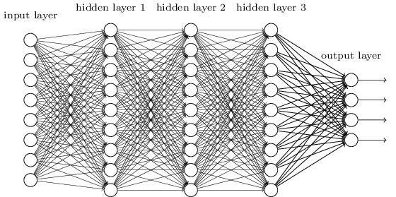
Example of neural network with 3 hidden layers.
Image from neuralnetworksanddeeplearning.com
The structure of a neural network is a series of layers, each with multiple nodes. The nodes of each layer are connected to all nodes of the previous layer. However, not all of these connections are equally strong. When training a neural network, some of these connections are made stronger or weaker as needed to statisfy the goals of the user. In our cause, we desire to minimize the error associated with the network's prediction (male vs female) as compared to the true classification. The specifics of how this is done will be discussed throughout this notebook.
Import Libraries
import obj
import numpy as np
import pandas as pd
import matplotlib.pyplot as plt
import seaborn as sns

# Parameters
sns.set_style('whitegrid')  # set plot backgrounds to white

# Set graphics to appear inline with notebook code
%matplotlib inline
Import scaled data from previous notebook.
data_scale = obj.load('var/data_scale')
Convert data to matrix form
Unlike the machine learning libraries in Sci-Kit Learn, Google's Tensorflow does not understand data in the form of our powerful Pandas DataFrames, therefore our data must be converted to a more basic matrix/array format.
# Convert features to matrix
feat_scale_array = data_scale.drop('label',axis=1).as_matrix()

print(feat_scale_array[0])
# Convert labels to array
label_array = data_scale['label'].as_matrix()

# Show label array in string format
print(label_array[:4])
print(label_array[-4:])
Convert label strings to binary targets
Further, the neural network system does not work directly with strings. Predictions from a neural network are not verbal declarations, but are very simply the "intensity" of the output nodes. In our specific case, we are trying to classify voices as either male or female. Therefore, our output layer will consist of simply two nodes, one to respresent a male classification, and one to represent a female classification. In all cases, both nodes will "light up", but in a well-trained model, one will be much "brighter" than the other, thus giving us our prediction.
To make our targets compatible with our neural network, we will encode the "male" string to match up with the first output node, and the "female" string to match up with the second. Notice how the output compares to the string output above.
#  "male"  --> [0,1]
# "female" --> [1,0]

target_array = []

for label in label_array:
    if label == 'male':
        target = [0,1]
    else:
        target = [1,0]
    target_array.append(target)

# Show target array in binary format
print(target_array[:4])
print(target_array[-4:])
Split data into testing and training sets
As always, it is necessary to separate our data into a set that will train our network, and a separate set to test the final fit.
from sklearn.model_selection import train_test_split

X_train, X_test, y_train, y_test = train_test_split(feat_scale_array, target_array,
                                                    test_size=0.33)
import tensorflow as tf

# Learning Parameters
rate   =  0.025  # training rate
epochs = 99      # number of full training cycles
batch  = 10      # number of data points to train per batch

# Network Parameters
n_hidden_1 = 10  # number of nodes in hidden layer 1
n_hidden_2 = 10  # number of nodes in hidden layer 2
n_hidden_3 = 10  # number of nodes in hidden layer 3
n_input    = len(feat_scale_array[0])  # 20
n_classes  = 2
n_samples  = len(X_train)  # 2122
Create network model
The mathematics behind neural networks are based on matrix arithmetic and manipulation. But against typical expectations, Tensorflow systems do not carry out their actions when they are defined. Instead, they are put into place and only run when called within a Tensorflow session.
When building our system, we will use Tensorflow's linear algebra methods to create our system, meaning that all the interactions will be defined upfront, but will not be executed until we call them to action later on.
def multilayer_perceptron(X, weights, biases):

    # Hidden Layer 1
    layer1 = tf.matmul(X, weights['w1'])
    layer1 = tf.add(layer1, biases['b1'])
    layer1 = tf.nn.relu(layer1)

    # Hidden Layer 2
    layer2 = tf.matmul(layer1, weights['w2'])
    layer2 = tf.add(layer2, biases['b2'])
    layer2 = tf.nn.relu(layer2)

    # Hidden Layer 3
    layer3 = tf.matmul(layer2, weights['w3'])
    layer3 = tf.add(layer3, biases['b3'])
    layer3 = tf.nn.relu(layer3)

    # Output Layer
    out = tf.matmul(layer3, weights['out'])
    out = tf.add(out, biases['out'])

    return out
Define inputs
Because we are only building the system and not asking it to perform work, our input values will be placeholders. We will define their type and shape upfront so that Tensorflow knows what it is working with.
# Define input and output
X = tf.placeholder('float', [None,n_input])
y = tf.placeholder('float', [None,n_classes])

# Define weights used to initialize the neural node connections
weights = {
    'w1' : tf.Variable(tf.random_normal([n_input,    n_hidden_1])),
    'w2' : tf.Variable(tf.random_normal([n_hidden_1, n_hidden_2])),
    'w3' : tf.Variable(tf.random_normal([n_hidden_2, n_hidden_3])),
    'out': tf.Variable(tf.random_normal([n_hidden_3, n_classes ]))
}

# Define some initial biases for the network to work against
biases = {
    'b1' : tf.Variable(tf.random_normal([n_hidden_1])),
    'b2' : tf.Variable(tf.random_normal([n_hidden_2])),
    'b3' : tf.Variable(tf.random_normal([n_hidden_3])),
    'out': tf.Variable(tf.random_normal([n_classes ]))
}

# Place inputs into model
model = multilayer_perceptron(X, weights, biases)
Define cost function and minimization function
The cost function is how our system knows how well or how poorly it is achieving its goal. A high cost signifies a large discrepancy between our output nodes' prediction and our target. A low cost signifies more agreement between the node outputs and our targets.
Because we want the cost function to be as small as possible, we will shape our network with a minimization function. A minimization function propogates through the network and changes the weighted strengths of the neural node connections in an effort to create a better predictive system.
# Define cost function
f_cost = tf.reduce_mean(tf.nn.softmax_cross_entropy_with_logits(model, y))

# Define minimization function
f_optimizer = tf.train.AdamOptimizer(learning_rate=rate).minimize(f_cost)
Run Network
Now that our network structure is built, our inputs are defined, and our training functions are defined, we are ready to run a Tensorflow session to put these pieces into motion.
# Define startup task
init = tf.initialize_all_variables()

# Instantiate session
s = tf.InteractiveSession()

# Start session
s.run(init)

# TRAIN NETWORK
for epoch in range(epochs):

    cost_avg = 0.

    batch_total = int(n_samples/batch)

    count = 0
    for batch_i in range(batch_total):
        X_batch_i = X_train[count : count+batch]
        y_batch_i = y_train[count : count+batch]
        count += batch

        _, cost = s.run([f_optimizer,f_cost], feed_dict={X:X_batch_i, y:y_batch_i})

        cost_avg += cost / batch_total

    print('Epoch {:2}:  cost = {:.20f}'.format(epoch+1, cost_avg))

print('\n')
print('Model trained successfully!')
Evaluate performance
With our network trained, it is time to evaluate how successfully it can classify our testing set of data.
# Define success
correct_target = tf.equal(tf.argmax(model, 1), tf.argmax(y, 1))
correct_target = tf.cast(correct_target, 'float')

# Define accuracy calculation
accuracy = tf.reduce_mean(correct_target)

# Find and print model accuracy
print('Accuracy is {:.2f}%'.format(100*accuracy.eval({X:X_test, y:y_test})))
Conclusion
Given the complexity of creating a neural network, one might expect unbeatable results for any given problem. However, as mentioned at the beginning of this notebook, the strength of neural networks is classifying very large and very complicated sets of data. Our data is fairly small, and not entirely complex. If we were dealing with a much more complicated set of data, then our other methodologies would likely perform below our standards and the neural network would prove indispensable.
But given our relatively small set of data, the neural network proved moderately successful.