Gender Recognition by Voice | 04 | Random Forest
Random Forest Method Overview
The random forest classification method is an example of a tree-based prediction algorithm. In general, tree-based prediction models aim to segment the data field by creating rules to segment each feature of the data. Then, to determine the class of a new sample of data, the sample is placed in the field according to the values of its features and is classified as appropriate for the field segment in which it falls.
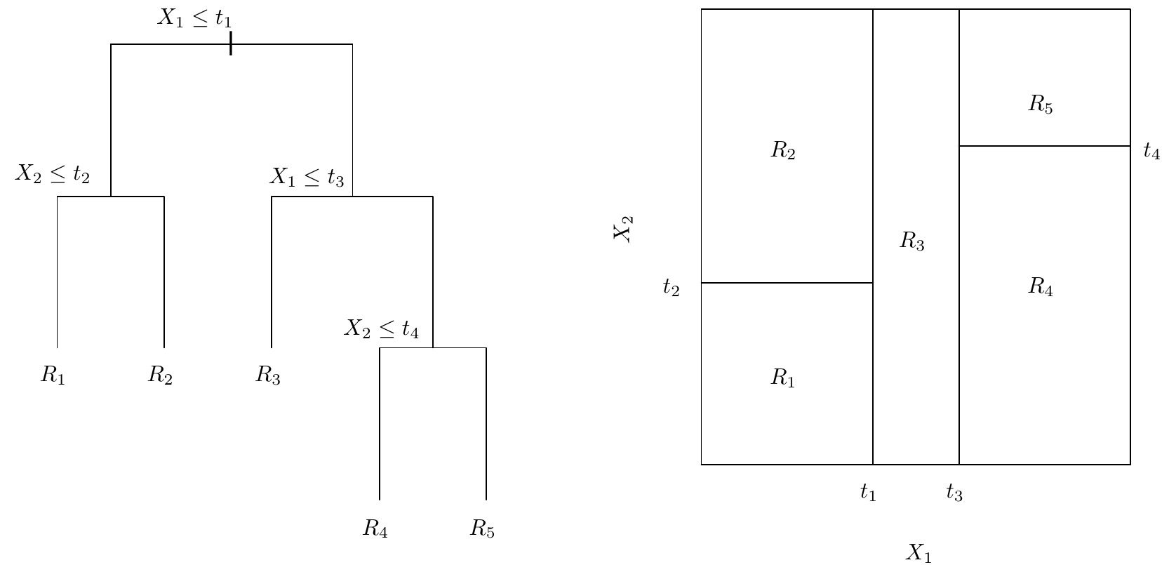
The plot on the left shows the decision tree used to classify a particular set of data. The plot on the right illustrates how the resulting segments separate the data field.
Image from An Introduction to Statistical Learning, Sixth Printing (Figure 8.3)
As you can imagine, tree methods are highly readable. The logic behind the final classification can be understood by observing which values the algorithm decided to place the segment barriers. However, simple tree methods are much less accurate compared to other methods, and must be enhanced with further complexities in order to come to par. Unfortunately, this comes at a cost to overall readability.
Tree enhancement is usually done by aggregating many decision trees together, and then "pruning" some of the unwanted complexity. Obtaining many trees is done by simply assigning each tree is own random sampling of the trainging data. Although they use the same data set, the segment positions of each tree are highly variant. To aggregate the trees, their segment position values are averaged, yielding a much more invariant result.
Import Libraries
import obj
import numpy as np
import pandas as pd
import matplotlib.pyplot as plt
import seaborn as sns

# Parameters
sns.set_style('whitegrid')  # set plot backgrounds to white

# Set graphics to appear inline with notebook code
%matplotlib inline
Import scaled data from prior notebook.
data_scale = obj.load('var/data_scale')
Split data into Training set and Testing Set
Like before, it is important to separate our data into a set used to train the classification model, and a set used to evaluate the model.
from sklearn.model_selection import train_test_split

X_train, X_test, y_train, y_test = train_test_split(data_scale.drop('label',axis=1), data_scale['label'],
                                                    test_size=0.33)
Create Random Forest model and determine best parameters
As discussed in the Overview, our Random Forest model will be the aggregate of many individual trees and not a single tree trained on all the data. This will reduce variance, but increase complexity. However, a well-pruned tree can avoid being too complex while still providing strong predictive capabilities.
from sklearn.ensemble import RandomForestClassifier

error_rate = []
nvals = range(1,202,5) # test a range of total trees to aggregate

for i in nvals:
    rfc = RandomForestClassifier(n_estimators=i)
    rfc.fit(X_train,y_train)
    y_pred_i = rfc.predict(X_test)
    error_rate.append(np.mean(y_pred_i != y_test))
Find optimal value
After training our model with different numbers of estimators, we can see what number of estimators is best for this task.
Additionally, we can see that there are diminishing returns as the number of estimators increases. When creating classification systems, it is important to understand its use case in order to best determine the time/complexity/accuracy tradeoffs that can be made. Always aiming for perfect accuracy may not be pracitical in situations where speed or understandability are also important.
plt.plot(nvals, error_rate, color='blue', linestyle='dashed', marker='o',
         markerfacecolor='red', markersize=10)
plt.title('Error Rate vs. Number of Predictors')
plt.xlabel('Number of Predictors')
plt.ylabel('Error Rate')

# Determine location of best performance
nloc = error_rate.index(min(error_rate))
print('Lowest error of %s occurs at n=%s.' % (error_rate[nloc], nvals[nloc]))

Create model using best parameters and evaluate performance
Using the optimal number of estimators, we will run the analysis again and proceed to quantify our classification accuracy.
# Instantiate model with optimal number of estimators
rfc = RandomForestClassifier(n_estimators=nvals[nloc])

# Fit model to training data
rfc.fit(X_train,y_train)

# Create preditions from test data
y_pred = rfc.predict(X_test)

# Run classification metrics
from sklearn.metrics import classification_report, confusion_matrix

print('Confusion Matrix:')
print(confusion_matrix(y_test, y_pred))
print('\n')
print('Classification Report:')
print(classification_report(y_test, y_pred))
Conclusion
Our Random Forest classifier has done a good job of differentiating between the different voices, outperforming our K Nearest Neighbors model. Typically, tree methods are inferior for classifing most types of data, but are useful in creating human-readable results. In this case, however, it seems that the data is well-suited to our Random Forest model.
Finally, we will see if a Neural Network will be able to provide even better results.